1. EDA & 전처리
들어가며
천체 유형 분류 대회
배경
안녕하세요 여러분! 천체 유형 분류 대회에 오신 것을 환영합니다.
최근 인류에게 다가온 빅데이터라는 단어는 우주와 천문학에게 낯설지 않습니다. 찰나의 순간에도 우주는 천문학적인 양의 데이터를 생산해왔고, 오래 전부터 천문학자들은 우주를 관측했으며 그 방대함에 비례하는 데이터를 수집 및 분석했기 때문입니다.
슬론 디지털 천체 관측(Sloan Digital Sky Survey: 이하 SDSS)는 세계적 천체 관측 프로젝트로, 우주에 대한 천문학적인 규모의 데이터를 수집하고 있습니다. 이곳에서 수집한 데이터는 약 6,000개 논문에 사용되었고, 25만 회 이상 인용되었을 정도로 천문학에 큰 기여를 했습니다. 점점 거대해지는 규모에 따라 데이터 처리에는 머신러닝과 딥러닝 기법이 활용되기 시작했습니다.
여전히 우주에는 다양한 미지의 이야기가 남아있고, 오늘날 인간은 하늘에서 많은 데이터를 얻어낼 정도로 발전했습니다. 이 데이터를 분석하여 어쩌면 드러나지 않은 규칙이 여러분의 손끝에서 밝혀질 수 있습니다. 새로운 알고리즘을 통해 우주의 비밀을 찾아주세요!
목적
천체 유형 분류 알고리즘 개발
EDA
#필요한 라이브러리 호출
import pandas as pd
import numpy as np
import matplotlib.pyplot as plt
import seaborn as sns

#훈련 및 테스트를 위한 데이터
train = pd.read_csv("./dataset_dsob/train.csv")
test = pd.read_csv('./dataset_dsob/test.csv')
sample_submission = pd.read_csv('./dataset_dsob/sample_submission.csv')
data info
#데이터 크기 확인
print('Size of train data', train.shape)
print('Size of test data', test.shape)

#데이터 요약정보 확인
train.info()
train.describe()


개별 변수 탐색
Type
#개별변수 탐색-type
#type별 개수 확인 - 전체 분포
plt.figure(figsize=(15,6))

plt.title('Type count')
plt.ylabel('count')
plt.xlabel('Type')
plt.bar(train.groupby('type')['fiberID'].count().index, train.groupby('type')['fiberID'].count().values)
plt.xticks(rotation=90)
plt.show()
#type별 개수 확인 - 실제 개수
train['type'].value_counts()
-> 클래스 불균형 심한 편임 => 별다른 조치가 필요하다
fiberId
#fiberId
sns.barplot(train['fiberID'].value_counts().index,train['fiberID'].value_counts())
plt.xticks(rotation=90);
-> 전체적인 분포를 살피고자, FiberId 하나의 값당 개수를 알려고 했는데 실패.. => 막대그래프 말고 산점도를 그려보자!
sns.set_style(style='whitegrid')

sns.scatterplot(
    data=train['fiberID'],
    x=train['fiberID'],
    y=train['fiberID'].value_counts(),
    palette='Paired_r'
    )

plt.title('fiberID\'s counts')
plt.xlabel('fiberID')
plt.ylabel('counts')
plt.legend(bbox_to_anchor=(1.05, 1), loc='upper left', borderaxespad=0)
-> 대개 600번대 이내로 몰려있음을 알 수 있다
type을 분석해봤을 때 QSO에 클래스가 몰려있던 것처럼 fiberID도 좀 더 세부적으로 살펴보고자 하였다.
type-fiberID
*코드 참고(https://github.com/Leewongi0731/DACON_CelestialClassification/blob/master/celestial_classifier.ipynb)
# type_num 열을 생성

column_number = {}
for i, column in enumerate(sample_submission.columns):
    column_number[column] = i

def to_number(x, dic):
    return dic[x]

train['type_num'] = train['type'].apply(lambda x: to_number(x, column_number))


#fiberID와 type 간의 상관관계
#type, fiberID관의 관계도를 보기위한 시각화

fig , ax = plt.subplots(nrows = len(set(train['type'])), ncols=1, figsize = (15,40))
for i in range(len(set(train['type']))):
    ax[i].scatter(train.loc[train['type_num']==i, 'fiberID'],range(train.loc[train['type_num']==i, 'fiberID'].shape[0]))
    ax[i].set_xlim(0,1000)
    ax[i].set_ylabel('count')
    ax[i].set_xlabel('fiberID')
    ax[i].set_title(list(column_number.keys())[i])

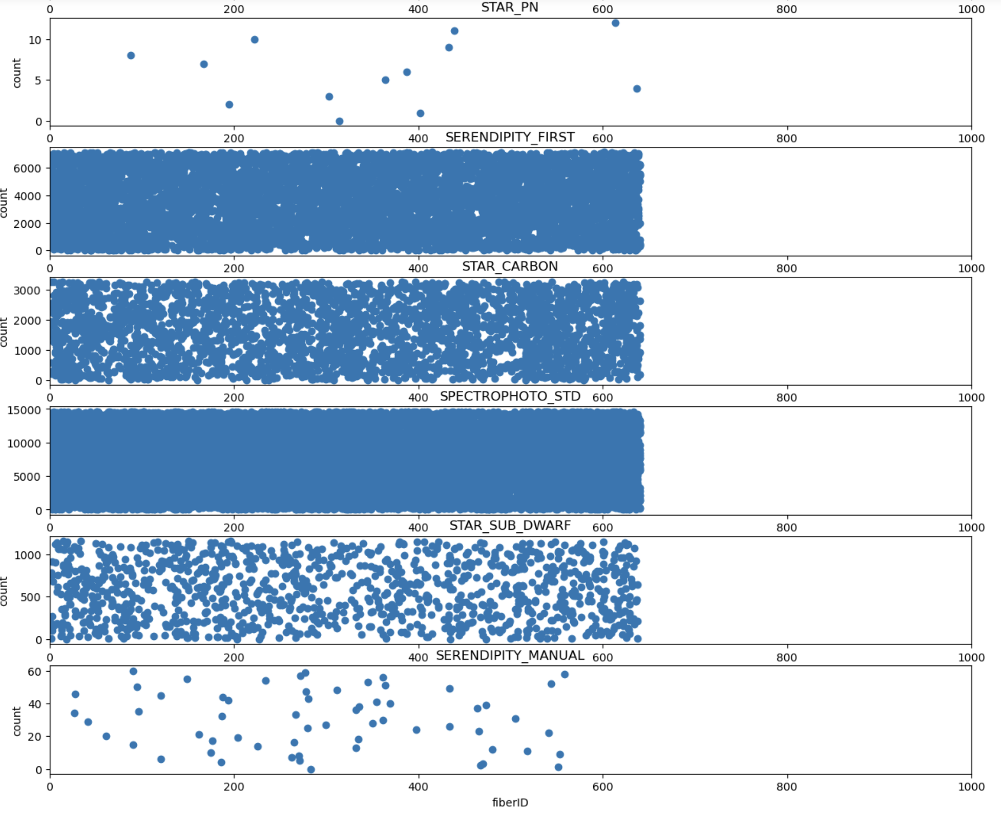
-> qso제외 나머지 첸체의 fiberId는 0에서 600번대 사이에 존재
정확한 fiberID 구분기준을 알아보자
#fiberId 구분기준(지점) 찾기,최댓값찾기 활용
train.groupby('type')['fiberID'].max()
-> 최댓값찾기 활용 => qso- 1000, 나머지 640
=> 분류되는 지점이 fiberId가 640일 때임을 알 수 잇음
한 번 더 확인한 결과 FiberID > 640인 천체는 QSO뿐임
train[ train['fiberID'] > 640 ]['type'].value_counts()
-> 향후 분류할 때 신경써야 할 부분인듯함
전처리
이상치 탐색
fig, ax = plt.subplots(nrows = 20, ncols= 1 ,figsize = (20,70))

for i in range(20):
    ax[i].scatter(x =  train.index, y = train[train.columns[i+2]].values)
    ax[i].set_title(train.columns[i+2])

plt.show()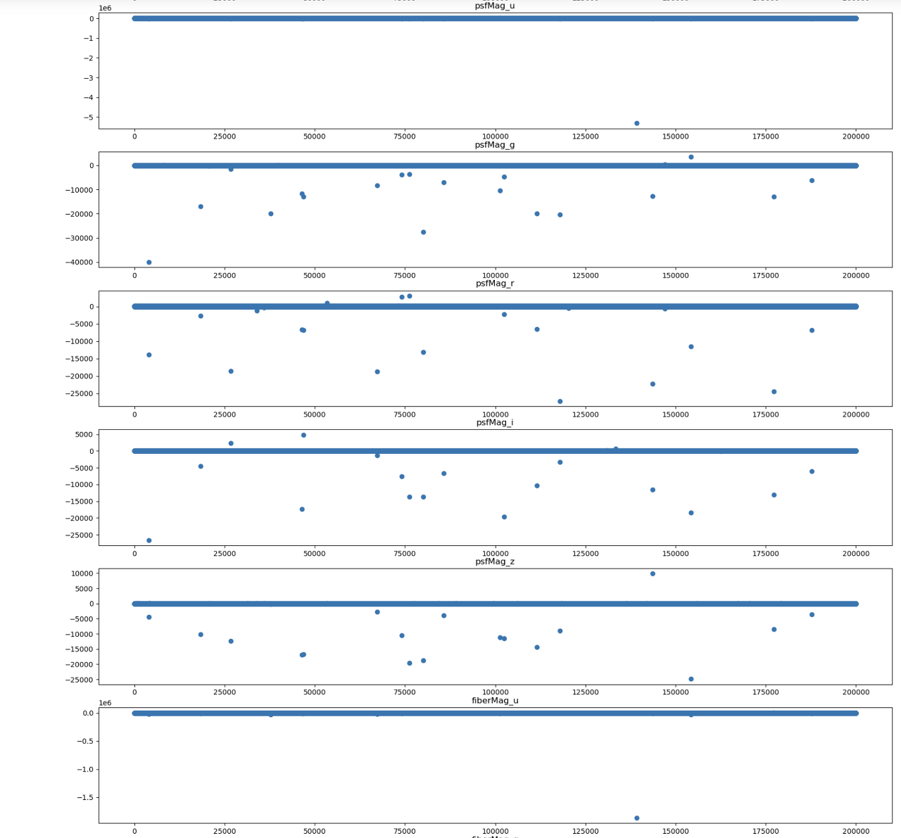


-> 대개의 값이 한 값에 몰려있지만, 극단적으로 떨어져있는 이상치가 꽤나 존재함 => 일부는 제거의 필요성 있음
type별 이상치 탐색 - boxplot활용
columns = train.columns
for s_type in columns[3:]:
    plt.figure(figsize=(18,3))
    sns.boxplot(x=train['type'],y=s_type,data=train)
    plt.title(s_type)
    plt.xticks(rotation=-90)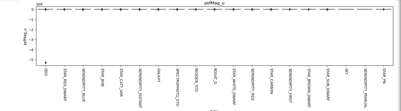
-> 이렇게 한 두 개 존재하는 컬럼의 경우 큰 문제가 되지 않지만


이렇게 다수 개가 있는 경우는 제거해줘야 한다고 판단됨
이상치 기준 선정을 위해 각 컬럼의 최대 , 최소값 확인
for col in train.columns[3:]:
    print(col,train[col].max())
    print(col,train[col].min())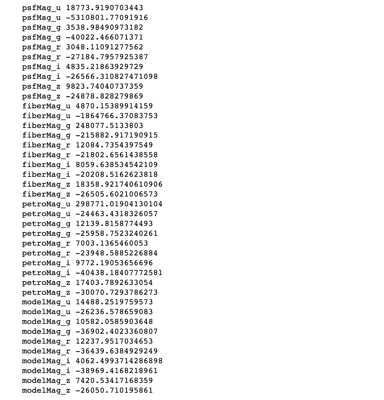
그런데 최대, 최소만으로 이상치 기준 선정하기 어려워서 100,200,300,400,500 ~ 1000까지 하나씩 넣어가며 그 때의 개수를 파악해봄
for col in train.columns[3:]:
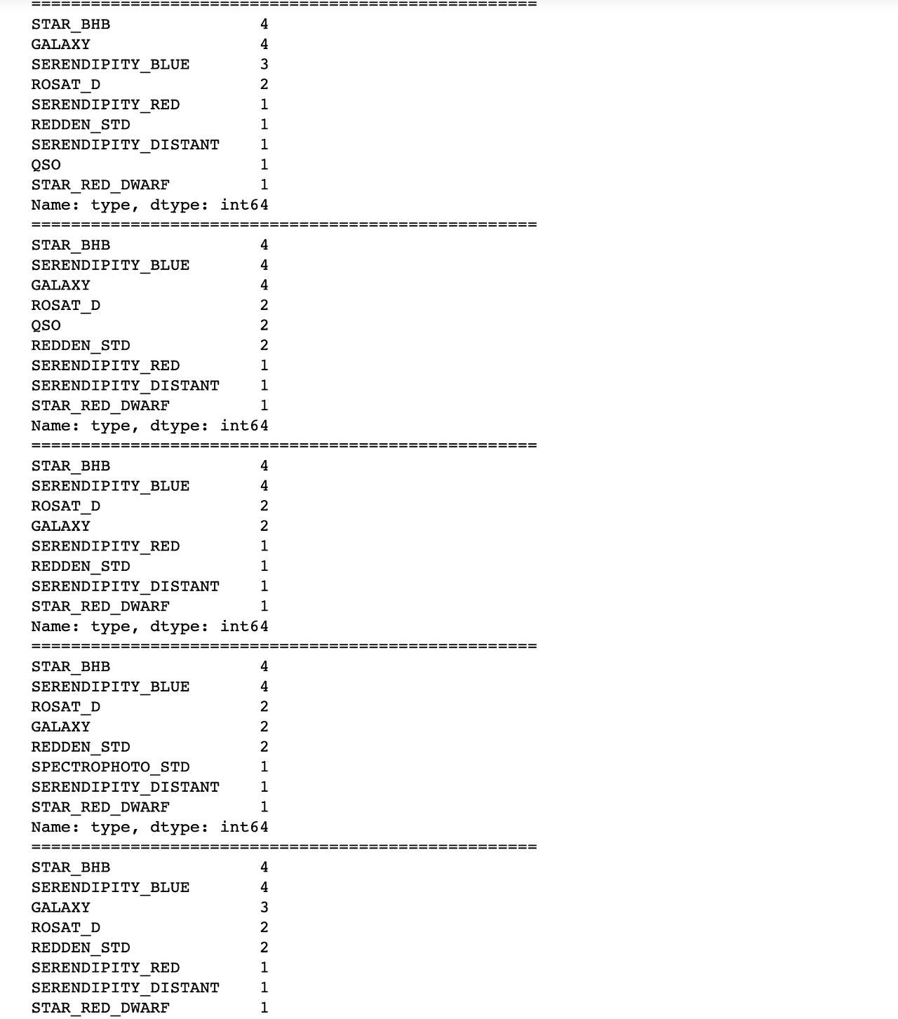
print(train[ abs(train[col]) > 500 ]['type'].value_counts())
print('===================================================')
100,200,300은 해당 범위가 너무 좁아 이상치 개수가 많았고, 1000이나 2000은 범위가 너무 넓어 이상치 개수 적었음
500~ 800은 해봤을 때 비슷한 정도로 나와 500을 이상치 기준 수치로 선정
그리고 제거해줌
remove_outlier_list = []

for i in range(len(train.index)):
    cnt = 0
    for j in train.columns[2:22]:
        if(abs(train.loc[i,j]) > 500):
            cnt += 1
            if cnt > 5:
                remove_outlier_list.append(i)
                break

print(remove_outlier_list)
-> 각 컬럼마다 500 넘는 값이 5 개 이상인 경우 제거 리스트에 담아줌
#이상치 값 제거한 새로운 데이터프레임 생성
train_c = train.drop(remove_outlier_list)

#이상치 제거 후 비교를 위한 시각화
fig, ax = plt.subplots(nrows = 20, ncols= 1 ,figsize = (20,70))

for i in range(20):
    ax[i].scatter(x =  train_c.index, y = train_c[train_c.columns[i+2]].values)
    ax[i].set_title(train_c.columns[i+2])


-> y축 범위를 확인해보면 대부분이 이상치가 제거된 것을 알 수 있지만, 애초에 이상치 개수가 적었던 'psfMag_u'와 같은 경우 이상치가 거의 제거되지 않음이 보임. 그렇지만 후에 영향을 크게 줄 것들은 제거했으므로 넘어감
모델링
학습을 위해 train_c 데이터의 type을 숫자형으로 변환
column_number = {}
for i, column in enumerate(sample_submission.columns):
    column_number[column] = i

def to_number(x, dic):
    return dic[x]

train_c['type_num'] = train_c['type'].apply(lambda x: to_number(x, column_number))
train_c['type_num']
사용할 모델인 xgboost 불러와줌
#모델링
from xgboost import XGBClassifier
import xgboost as xgb
from xgboost import plot_importance
from sklearn.model_selection import train_test_split
from sklearn.metrics import accuracy_score, precision_score, recall_score, confusion_matrix, roc_auc_score, f1_score
학습 데이터
x = train_c.drop(['type_num','type'],axis = 1) #column접근
y = train_c['type_num'].values
test_x = test
RANDOM_SEED = 2000 #random_state와 일치
x_train, x_valid, y_train, y_valid = train_test_split(x, y, \
test_size=0.2, random_state=RANDOM_SEED, stratify = y)xgb_clf = XGBClassifier(booster='gbtree',
silent=True,
max_depth=5,
min_child_weight=8,
gamma=1,n_estimators=100,
colsample_bytree=0.6,
colsample_bylevel=0.6,
objective='multi:softprob',
random_state=RANDOM_SEED)
xgb_clf.fit(x_train,y_train, eval_set=[(x_train, y_train), (x_valid, y_valid)])파라미터 설정해줌
- gbtree -> gblinear보다 트리가 적합하다고 생각되어 선택


에측결과 확인
xgb_pred = xgb_clf.predict_proba(test_x)

print(np.round(xgb_pred[:5], 3))
우선 5 개만 뽑아서 봤는데 잘 된 건지 모르겠다
피처 중요도 시각화
%matplotlib inline

fig, ax = plt.subplots(figsize=(10, 12))
plot_importance(xgb_clf, ax=ax)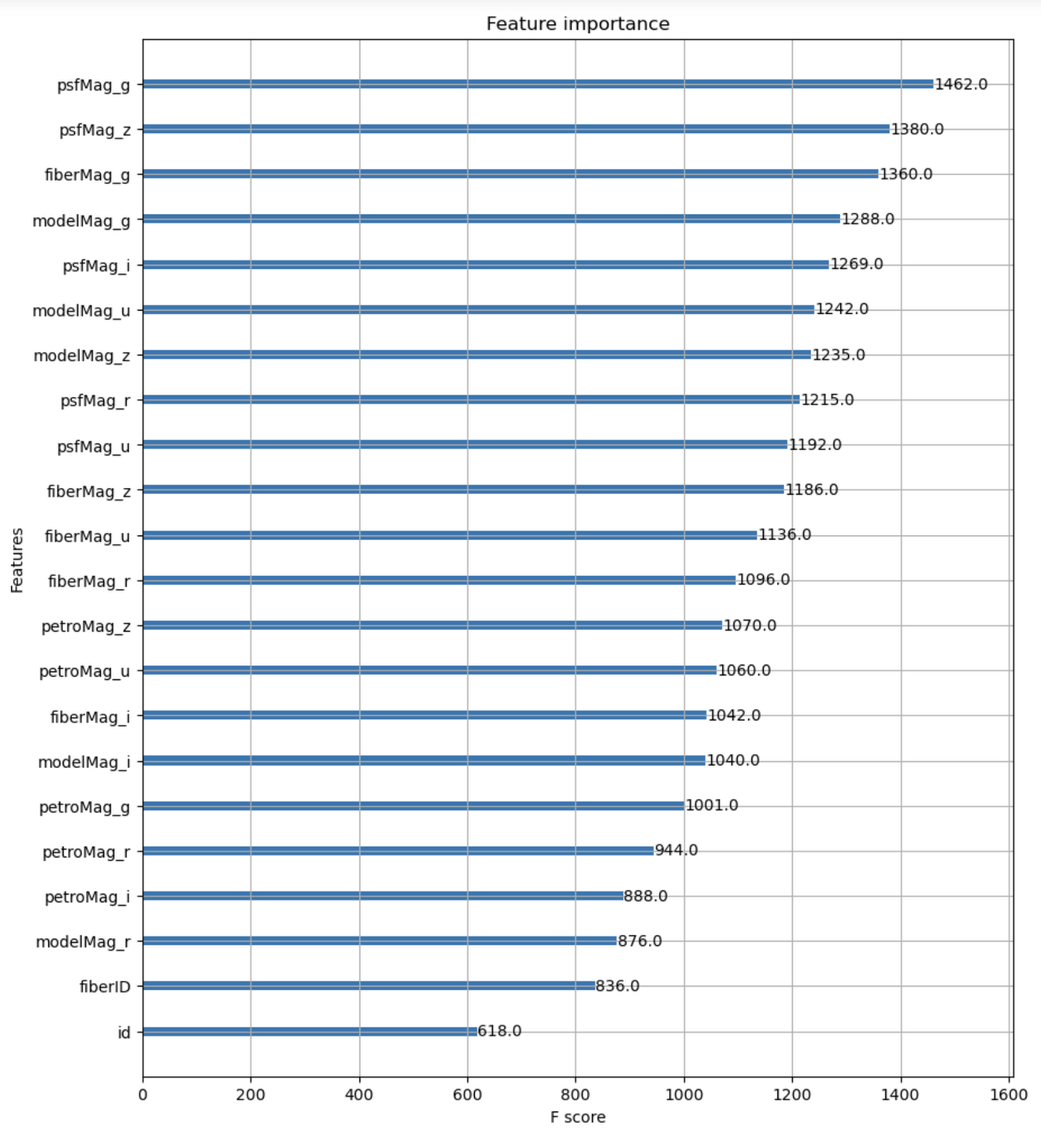
출처
https://dacon.io/competitions/official/235573/codeshare/694?page=1&dtype=recent
https://dacon.io/competitions/official/235573/talkboard/400609
https://velog.io/@leo_kim/부스팅-계열-앙상블-알고리즘
https://youtu.be/8b1JEDvenQU
https://youtu.be/GrJP9FLV3FE
https://teddylee777.github.io/scikit-learn/scikit-learn-ensemble/
https://hwi-doc.tistory.com/entry/이해하고-사용하자-XGBoost
[ML] XGBoost 이해하고 사용하자
순서 개념 기본 구조 파라미터 GridSearchCV 1. 개념 'XGBoost (Extreme Gradient Boosting)' 는 앙상블의 부스팅 기법의 한 종류입니다. 이전 모델의 오류를 순차적으로 보완해나가는 방식으로 모델을 형성하
hwi-doc.tistory.com
https://github.com/Leewongi0731/DACON_CelestialClassification/blob/master/celestial_classifier.ipynb
'💡 WIDA > DACON 분류-회귀' 카테고리의 다른 글
| [DACON/김경은] 프로젝트 에세이 (4) | 2023.05.05 |
|---|---|
| [DACON/김세연] 프로젝트 에세이 (4) | 2023.05.05 |
| [DACON/참고자료] 앙상블 모델 (0) | 2023.05.01 |
| [DACON/참고자료] SVM 참고자료 (0) | 2023.04.26 |
| [DACON/최다예] 파이썬을 이용한 EDA (0) | 2023.04.07 |